Logistic Regression

This is for classification problems, rather than regression problems.

Rather than our output vector $y$ being a continuous range of values, it's only 0 or 1.

Hypothesis Representation

We could try to use linear regression and map predictions greater than 0.5 as 1, and all less than 0.5 as 0. However this doesn't work well because classification isn't linear.

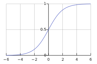
Instead, we use the Sigmoid, or logistic, function:

\[ \begin{align*} & h_\theta(x) = g(\theta^Tx) \\ & z = \theta^Tx \\ & g(z) = \dfrac{1}{1 + e^{-z}} \end{align*} \]

This gives us the probability that our output is 1.

Decision Boundary

In order to transform our $0 \leq h_\theta(x) \leq 1$ output to a discrete value, we classify $\geq 0.5$ as $y = 1$.

The logistic function gives an output $\geq 0.5$ when it's input is $\geq 0$.

So if we have input $\theta^TX$, that means:

\[h_\theta(x) = g(\theta^Tx) \geq 0.5 \\ when \ \theta^Tx \geq 0\]

From this, we can say:

\[\theta^Tx \geq 0 \rightarrow y = 1 \\ \theta^Tx \lt 0 \rightarrow y = 0\]

The decision boundary is the line that separates the area where $y=0$ and where $y=1$.

Cost Function

If we use the same cost function as we use for linear regression, the output will be wavy due to use of the sigmoid function as the hypothesis function.

Instead, we want the cost function to be a logarithmic function that has high cost when the hypothesis is wrong, and low cost when it's right. The algorithm has a high cost for getting the classification wrong with high confidence - the cost approaches infinity.

\[ Cost( h_\theta(x), y)) = -log(h_\theta(x)) \ \text{if y = 1} \\ Cost(h_\theta(x, y)) = -log(1-h_\theta(x)) \ \text{if y = 0} \]

Simplified Cost Function and Gradient Descent

We can compress the above conditional cost function into one case:

\[ Cost(h_\theta(x),y) = -y \; log( h_\theta(x)) - (1-y)log(1-h_\theta(x)) \]

When $y=1$, then the second term will be zero; when $y=0$ the first term will be zero.

For $\theta$, we can write the entire cost function:

\[ J(\theta) = - \frac{1}{m} \sum_{i=0}^m [ y^{(i)} log(h_\theta(x^{(i)})) + (1-y^{(i)}) log (1-h_\theta(x^{(i)})) ] \]

Gradient Descent

The general form of gradient descent is to repeat

\[\theta_j := \theta_j - \alpha \frac{\delta}{\delta \theta_j} J(\theta)\]

We can work out the derivative part using calculus to get

\[\theta_j := \theta_j - \frac{\alpha}{m} \sum_{i=1}^m (h_\theta(x^{(i)}) - y^{(i)}) x_j^{(i)}\]

A vectorised implementation of this is:

\[ \theta := \theta - \frac{\alpha}{m} X^T (g(X\theta) - \vec{y}) \]

Multi-class classification: One-vs-all

If we're trying to organise data into more than two categories, we expand our definition so that $y = {0,1,...,n}$.

We divide the problem into $n+1$ binary classification problems, and for each we predict the probability that $y$ is a member of one of our classes.

\[ h_\theta^{(0)}(x) = P(y=0|x;\theta) \\ h_\theta^{(1)}(x) = P(y=1|x;\theta) \\ ... \\ h_\theta^{(n)}(x) = P(y=n|x;\theta) \\ prediction = max_i(h_\theta^{(i)}(x)) \]

For each, we're taking one of the classes and putting all the others into a single second class. We do this repeatedly, and use the hypothesis that returned the highest value as our prediction.